Econometria: exemplo de dados em painel em R - Torres-Reyna data
Licença
This work is licensed under the Creative Commons Attribution-ShareAlike 4.0 International License. To view a copy of this license, visit http://creativecommons.org/licenses/by-sa/4.0/ or send a letter to Creative Commons, PO Box 1866, Mountain View, CA 94042, USA.

License: CC BY-SA 4.0
Citação
Sugestão de citação: FIGUEIREDO, Adriano Marcos Rodrigues. Econometria: exemplo de dados em painel em R - Torres-Reyna data. Campo Grande-MS,Brasil: RStudio/Rpubs, 2020. Disponível em http://rpubs.com/amrofi/Econometrics_panel_torres_reyna e em https://adrianofigueiredo.netlify.app/post/Econometrics_panel_torres_reyna/.
Script para reprodução (se utilizar, citar como acima)
Download 2020-05-04-Econometrics_panel_torres_reyna.RmdIntrodução
Este é um exercício para aula de econometria com dados em painel, adaptado a partir de Torres-Reyna (2010), Katchova (2013). UM exemplo de dados em painel pode ser visto em Figueiredo (2019, http://rpubs.com/amrofi/TS_dataset_types) como apresentado por Greene (2003), ou Greene (2012).
# Exemplo de Dados de Corte Transversal
library(tidyr)
library(dplyr)
library(DT)
library(magrittr)
library(plm)
library(systemfit)
Os dados em painel, ou de combinação de seção cruzada e série temporal (SCST), ou também chamados de dados longitudinais, associam dados de diferentes unidades ou indivíduos para diferentes períodos de tempo.
Segue o exemplo de Torres-Reyna (2010) para os dados em Panel101.dta, para 10 anos (1990-99) e 7 países (aqui designados pelas letras A até G):
library(foreign)
Panel <- read.dta("http://dss.princeton.edu/training/Panel101.dta")
datatable(Panel)
coplot(y ~ year | country, type = "l", data = Panel) # Linhas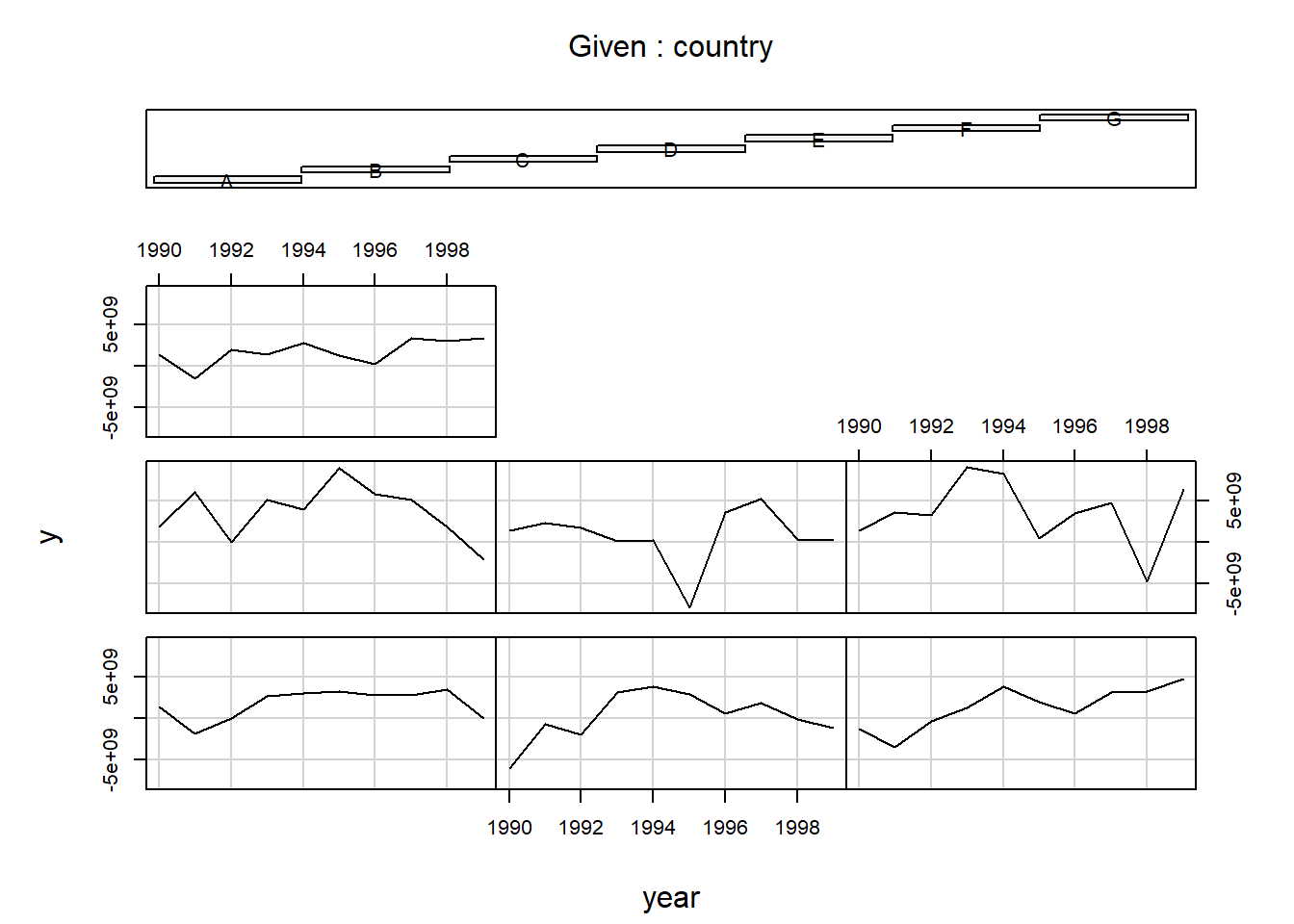
coplot(y ~ year | country, type = "b", data = Panel) # Pontos e linhas
# As barras ao topo indicam o gráfico correspondente a cada país, da esquerda
# para direita e de baixo para cima (Muenchen/Hilbe:355).
library(car)
scatterplot(y ~ year | country, boxplots = FALSE, smooth = TRUE, reg.line = FALSE,
data = Panel)
Modelo Empilhado (pooled OLS)
O modelo pooled, ou também chamado de dados empilhados, estimado por MQO (mínimos quadrados ordinários), será o mesmo que a estimação do modelo por MQO ignorando o formato de painel.
library(plm)
# options('scipen'=100, 'digits'=4)
Panel.set <- pdata.frame(Panel, index = c("country", "year"))
formula <- y ~ x1
# pooled OLS
pooled <- plm(formula, data = Panel.set, index = c("country", "year"), model = "pooling")
summary(pooled)
Pooling Model
Call:
plm(formula = formula, data = Panel.set, model = "pooling", index = c("country",
"year"))
Balanced Panel: n = 7, T = 10, N = 70
Residuals:
Min. 1st Qu. Median Mean 3rd Qu. Max.
-9.55e+09 -1.58e+09 1.55e+08 0.00e+00 1.42e+09 7.18e+09
Coefficients:
Estimate Std. Error t-value Pr(>|t|)
(Intercept) 1524319070 621072624 2.4543 0.01668 *
x1 494988914 778861261 0.6355 0.52722
---
Signif. codes: 0 '***' 0.001 '**' 0.01 '*' 0.05 '.' 0.1 ' ' 1
Total Sum of Squares: 6.2729e+20
Residual Sum of Squares: 6.2359e+20
R-Squared: 0.0059046
Adj. R-Squared: -0.0087145
F-statistic: 0.403897 on 1 and 68 DF, p-value: 0.52722# o mesmo que o OLS comum sem especificar painel
ols <- lm(y ~ x1, data = Panel)
summary(ols)
Call:
lm(formula = y ~ x1, data = Panel)

Residuals:
       Min         1Q     Median         3Q        Max
-9.546e+09 -1.578e+09  1.554e+08  1.422e+09  7.183e+09

Coefficients:
             Estimate Std. Error t value Pr(>|t|)
(Intercept) 1.524e+09  6.211e+08   2.454   0.0167 *
x1          4.950e+08  7.789e+08   0.636   0.5272
---
Signif. codes:  0 '***' 0.001 '**' 0.01 '*' 0.05 '.' 0.1 ' ' 1

Residual standard error: 3.028e+09 on 68 degrees of freedom
Multiple R-squared:  0.005905,  Adjusted R-squared:  -0.008714
F-statistic: 0.4039 on 1 and 68 DF,  p-value: 0.5272
suppressMessages(library(stargazer))
stargazer(pooled, title = "Título: Resultado da Regressão Pooled OLS", align = TRUE,
type = "text", style = "all", keep.stat = c("aic", "bic", "rsq", "adj.rsq", "n"))
Título: Resultado da Regressão Pooled OLS
========================================
                 Dependent variable:
             ---------------------------
                          y
----------------------------------------
x1                 494,988,914.000
                  (778,861,261.000)
                      t = 0.636
                      p = 0.528
Constant         1,524,319,070.000**
                  (621,072,624.000)
                      t = 2.454
                      p = 0.017
----------------------------------------
Observations             70
R2                      0.006
Adjusted R2            -0.009
========================================
Note:        *p<0.1; **p<0.05; ***p<0.01
# plot do MQO
yhat <- ols$fitted
plot(Panel$x1, Panel$y, pch = 19, xlab = "x1", ylab = "y")
abline(lm(Panel$y ~ Panel$x1), lwd = 3, col = "red")
É possível estimar com erros-padrõesrobustos conforme Arellano e ainda com erros-padrões consistentes de White (principalmente paras as correlações cruzadas), analogamente ao realizado por Greene (2012, p.352), de modo a ter ideia do efeito de ignorar as características entre indivíduos e entre períodos.
# o modelo com erros-padrões robustos de Arellano
summary(pooled, vcov = function(x) vcovHC(x, method = "arellano"))
Pooling Model
Note: Coefficient variance-covariance matrix supplied: function(x) vcovHC(x, method = "arellano")
Call:
plm(formula = formula, data = Panel.set, model = "pooling", index = c("country",
"year"))
Balanced Panel: n = 7, T = 10, N = 70
Residuals:
Min. 1st Qu. Median Mean 3rd Qu. Max.
-9.55e+09 -1.58e+09 1.55e+08 0.00e+00 1.42e+09 7.18e+09
Coefficients:
Estimate Std. Error t-value Pr(>|t|)
(Intercept) 1524319070 890414623 1.7119 0.09147 .
x1 494988914 772694006 0.6406 0.52393
---
Signif. codes: 0 '***' 0.001 '**' 0.01 '*' 0.05 '.' 0.1 ' ' 1
Total Sum of Squares: 6.2729e+20
Residual Sum of Squares: 6.2359e+20
R-Squared: 0.0059046
Adj. R-Squared: -0.0087145
F-statistic: 0.41037 on 1 and 6 DF, p-value: 0.54545# o modelo com erros-padrões consistentes com heterocedasticidade de White
summary(pooled, vcov = function(x) vcovHC(x, method = "white1"))Pooling Model
Note: Coefficient variance-covariance matrix supplied: function(x) vcovHC(x, method = "white1")
Call:
plm(formula = formula, data = Panel.set, model = "pooling", index = c("country",
"year"))
Balanced Panel: n = 7, T = 10, N = 70
Residuals:
Min. 1st Qu. Median Mean 3rd Qu. Max.
-9.55e+09 -1.58e+09 1.55e+08 0.00e+00 1.42e+09 7.18e+09
Coefficients:
Estimate Std. Error t-value Pr(>|t|)
(Intercept) 1524319070 654083961 2.3305 0.02276 *
x1 494988914 680225903 0.7277 0.46931
---
Signif. codes: 0 '***' 0.001 '**' 0.01 '*' 0.05 '.' 0.1 ' ' 1
Total Sum of Squares: 6.2729e+20
Residual Sum of Squares: 6.2359e+20
R-Squared: 0.0059046
Adj. R-Squared: -0.0087145
F-statistic: 0.529523 on 1 and 6 DF, p-value: 0.49421Modelo de Efeitos Fixos (Fixed Effects - FE)
(Modelo Covariancia, Estimador ‘Within’, Modelo de variável dummy individual, Modelo Least Squares Dummy Variable (LSDV))
Use o modelo de efeitos fixos (FE para Fixed Effects) sempre que estiver interessado apenas em analisar o impacto de variáveis que variam ao longo do tempo. O FE explora a relação entre variáveis preditoras e o resultado dentro de uma entidade (país, pessoa, empresa, etc.). Cada entidade tem suas próprias características individuais que podem ou não influenciar as variáveis preditoras (por exemplo, ser homem ou mulher pode influenciar a opinião em relação à determinada questão ou o sistema político de um determinado país pode ter algum efeito sobre o comércio ou PIB; ou as práticas de negócios de uma empresa podem influenciar o preço de suas ações).
Ao usar o FE, supõe-se que algo dentro do indivíduo pode impactar ou viesar o preditor ou as variáveis de resultado e é preciso controlar isso.
Essa é a justificativa por trás da suposição da correlação entre o termo de erro da entidade e as variáveis preditoras. O FE remove o efeito dessas características invariantes no tempo, para que se avalie o efeito líquido dos preditores na variável de resultado.
Outra pressuposição importante do modelo FE é que essas características invariantes no tempo são exclusivas do indivíduo e não devem ser correlacionadas com outras características individuais. Cada entidade é diferente, portanto, o termo de erro da entidade e a constante (que captura as características individuais) não devem ser correlacionadas com as outras.
Se os termos de erros estão correlacionados, então o FE não é adequado, uma vez que as inferências podem não estar corretas e você precisa modelar essa relação (provavelmente usando efeitos aleatórios), esta é a principal razão para o teste de Hausman (apresentado mais adiante).
Heterogeneidade entre países
library(gplots)
plotmeans(y ~ country, main = "Heterogeneidade entre países", data = Panel)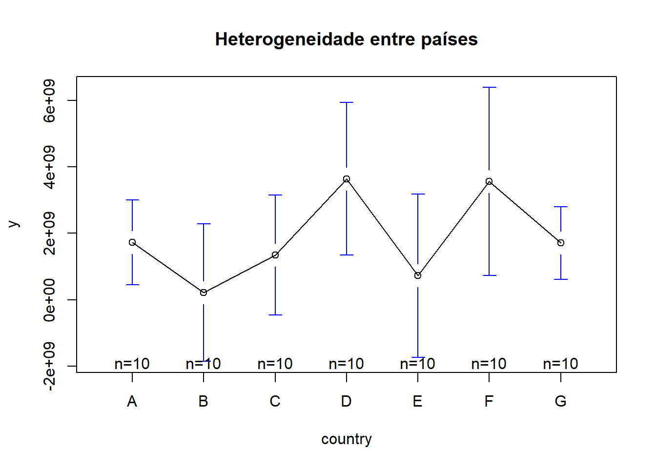
# plotmeans faz um intervalo de confiança de 95% em torno das médias
detach("package:gplots")
# detach remove o pacote ‘gplots’ do ambiente de trabalho
Heterogeneidade entre anos
library(gplots)
plotmeans(y ~ year, main = "Heterogeneidade entre anos", data = Panel)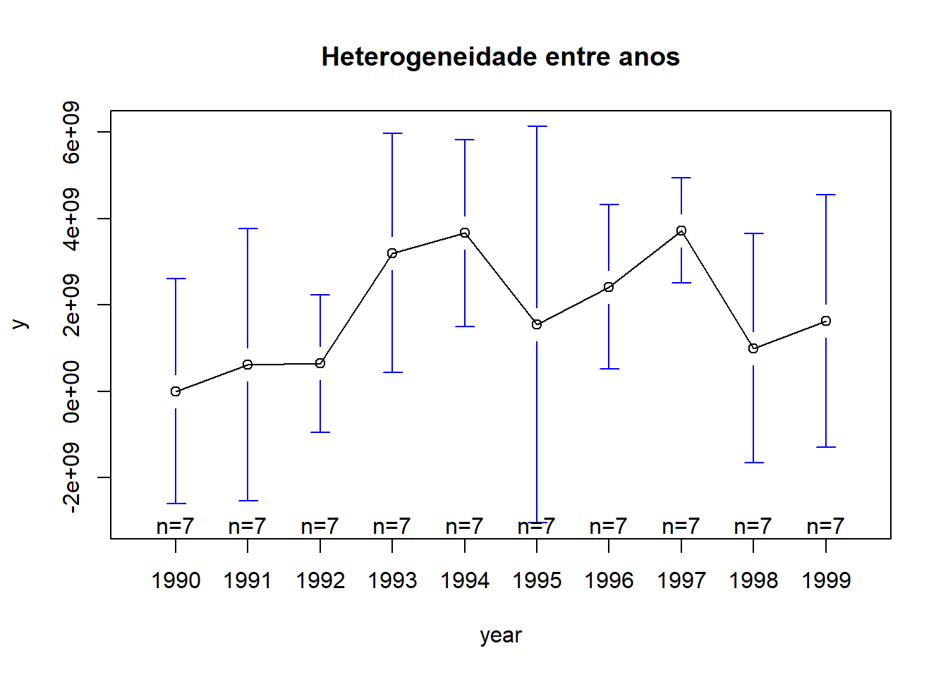
# plotmeans faz um intervalo de confiança de 95% em torno das médias
detach("package:gplots")
# detach remove o pacote ‘gplots’ do ambiente de trabalho
Operacionalização de outros modelos
Efeitos Fixos com Least squares dummy variable - LSDV
fixed.dum <- lm(y ~ x1 + factor(country) - 1, data = Panel)
summary(fixed.dum)
Call:
lm(formula = y ~ x1 + factor(country) - 1, data = Panel)

Residuals:
       Min         1Q     Median         3Q        Max
-8.634e+09 -9.697e+08  5.405e+08  1.386e+09  5.612e+09

Coefficients:
                   Estimate Std. Error t value Pr(>|t|)
x1                2.476e+09  1.107e+09   2.237  0.02889 *
factor(country)A  8.805e+08  9.618e+08   0.916  0.36347
factor(country)B -1.058e+09  1.051e+09  -1.006  0.31811
factor(country)C -1.723e+09  1.632e+09  -1.056  0.29508
factor(country)D  3.163e+09  9.095e+08   3.478  0.00093 ***
factor(country)E -6.026e+08  1.064e+09  -0.566  0.57329
factor(country)F  2.011e+09  1.123e+09   1.791  0.07821 .
factor(country)G -9.847e+08  1.493e+09  -0.660  0.51190
---
Signif. codes:  0 '***' 0.001 '**' 0.01 '*' 0.05 '.' 0.1 ' ' 1

Residual standard error: 2.796e+09 on 62 degrees of freedom
Multiple R-squared:  0.4402,    Adjusted R-squared:  0.368
F-statistic: 6.095 on 8 and 62 DF,  p-value: 8.892e-06
Between estimator (com variação)
between <- plm(formula, data = Panel.set, model = "between")
summary(between)
Oneway (individual) effect Between Model
Call:
plm(formula = formula, data = Panel.set, model = "between")
Balanced Panel: n = 7, T = 10, N = 70
Observations used in estimation: 7
Residuals:
A B C D E F
-407819091 -1758911755 62115802 1362404534 -1229066428 1692772511
G
278504427
Coefficients:
Estimate Std. Error t-value Pr(>|t|)
(Intercept) 2461785986 1092643022 2.2531 0.07399 .
x1 -951717959 1480461707 -0.6429 0.54864
---
Signif. codes: 0 '***' 0.001 '**' 0.01 '*' 0.05 '.' 0.1 ' ' 1
Total Sum of Squares: 1.0365e+19
Residual Sum of Squares: 9.5737e+18
R-Squared: 0.076342
Adj. R-Squared: -0.10839
F-statistic: 0.413259 on 1 and 5 DF, p-value: 0.54864First differences estimator
firstdiff <- plm(formula, data = Panel.set, model = "fd")
summary(firstdiff)
Oneway (individual) effect First-Difference Model
Call:
plm(formula = formula, data = Panel.set, model = "fd")
Balanced Panel: n = 7, T = 10, N = 70
Observations used in estimation: 63
Residuals:
Min. 1st Qu. Median Mean 3rd Qu. Max.
-9.09e+09 -1.92e+09 -4.71e+07 0.00e+00 1.73e+09 1.21e+10
Coefficients:
Estimate Std. Error t-value Pr(>|t|)
(Intercept) 112324037 459179084 0.2446 0.80757
x1 2332571239 1205546123 1.9349 0.05765 .
---
Signif. codes: 0 '***' 0.001 '**' 0.01 '*' 0.05 '.' 0.1 ' ' 1
Total Sum of Squares: 8.5496e+20
Residual Sum of Squares: 8.0552e+20
R-Squared: 0.057824
Adj. R-Squared: 0.042378
F-statistic: 3.74371 on 1 and 61 DF, p-value: 0.057647Fixed effects or within estimator
Oneway (individual) effect Within Model
fixed <- plm(formula, data = Panel.set, index = c("country", "year"), effect = c("individual"),
    model = "within")
summary(fixed)
Oneway (individual) effect Within Model
Call:
plm(formula = formula, data = Panel.set, effect = c("individual"),
model = "within", index = c("country", "year"))
Balanced Panel: n = 7, T = 10, N = 70
Residuals:
Min. 1st Qu. Median Mean 3rd Qu. Max.
-8.63e+09 -9.70e+08 5.40e+08 0.00e+00 1.39e+09 5.61e+09
Coefficients:
Estimate Std. Error t-value Pr(>|t|)
x1 2475617827 1106675594 2.237 0.02889 *
---
Signif. codes: 0 '***' 0.001 '**' 0.01 '*' 0.05 '.' 0.1 ' ' 1
Total Sum of Squares: 5.2364e+20
Residual Sum of Squares: 4.8454e+20
R-Squared: 0.074684
Adj. R-Squared: -0.029788
F-statistic: 5.00411 on 1 and 62 DF, p-value: 0.028892Efeitos fixos (one-way individual)
print(fixef(fixed)) A B C D E F
880542404 -1057858363 -1722810755 3162826897 -602622000 2010731793
G
-984717493 Oneway (time) effect Within Model
Agora alterando para conter efeitos fixos no tempo.
fixed.onet <- plm(formula = formula, data = Panel.set, index = c("country", "year"),
    effect = c("time"), model = "within")
summary(fixed.onet)
Oneway (time) effect Within Model
Call:
plm(formula = formula, data = Panel.set, effect = c("time"),
model = "within", index = c("country", "year"))
Balanced Panel: n = 7, T = 10, N = 70
Residuals:
Min. 1st Qu. Median Mean 3rd Qu. Max.
-9.47e+09 -1.56e+09 -7.39e+06 0.00e+00 1.48e+09 7.20e+09
Coefficients:
Estimate Std. Error t-value Pr(>|t|)
x1 -173111508 815529770 -0.2123 0.8326
Total Sum of Squares: 5.1406e+20
Residual Sum of Squares: 5.1367e+20
R-Squared: 0.00076311
Adj. R-Squared: -0.1686
F-statistic: 0.045058 on 1 and 59 DF, p-value: 0.83263summary(fixed.onet, vcov = function(x) vcovHC(x, method = "arellano"))Oneway (time) effect Within Model
Note: Coefficient variance-covariance matrix supplied: function(x) vcovHC(x, method = "arellano")
Call:
plm(formula = formula, data = Panel.set, effect = c("time"),
model = "within", index = c("country", "year"))
Balanced Panel: n = 7, T = 10, N = 70
Residuals:
Min. 1st Qu. Median Mean 3rd Qu. Max.
-9.47e+09 -1.56e+09 -7.39e+06 0.00e+00 1.48e+09 7.20e+09
Coefficients:
Estimate Std. Error t-value Pr(>|t|)
x1 -173111508 691358030 -0.2504 0.8032
Total Sum of Squares: 5.1406e+20
Residual Sum of Squares: 5.1367e+20
R-Squared: 0.00076311
Adj. R-Squared: -0.1686
F-statistic: 0.0626969 on 1 and 6 DF, p-value: 0.81064Efeitos fixos (one-way time)
fixef(fixed.onet) 1990 1991 1992 1993 1994 1995 1996
53946716 711200607 762927804 3292078022 3813870160 1664285774 2559291627
1997 1998 1999
3865882558 1125968837 1723033310 Two-ways (individual and time) effects Within Model
fixed.two <- plm(formula = formula, data = Panel.set, index = c("country", "year"),
    effect = c("twoways"), model = "within")
summary(fixed.two)
Twoways effects Within Model
Call:
plm(formula = formula, data = Panel.set, effect = c("twoways"),
model = "within", index = c("country", "year"))
Balanced Panel: n = 7, T = 10, N = 70
Residuals:
Min. 1st Qu. Median Mean 3rd Qu. Max.
-7.92e+09 -1.05e+09 -1.40e+08 0.00e+00 1.63e+09 5.49e+09
Coefficients:
Estimate Std. Error t-value Pr(>|t|)
x1 1389050354 1319849567 1.0524 0.2974
Total Sum of Squares: 4.1041e+20
Residual Sum of Squares: 4.0201e+20
R-Squared: 0.020471
Adj. R-Squared: -0.27524
F-statistic: 1.10761 on 1 and 53 DF, p-value: 0.29738Efeitos fixos (two-ways - individual and time)
fixef(fixed.two) A B C D E F G
1252552899 -499653716 -376476457 3372498854 -20764090 2690388678 196220903 Random effects estimator
Oneway (individual) effect Random Effect Model (Swamy-Arora’s transformation - default)
random <- plm(formula = formula, data = Panel.set, effect = c("individual"), model = "random")
summary(random)
Oneway (individual) effect Random Effect Model
(Swamy-Arora's transformation)
Call:
plm(formula = formula, data = Panel.set, effect = c("individual"),
model = "random")
Balanced Panel: n = 7, T = 10, N = 70
Effects:
var std.dev share
idiosyncratic 7.815e+18 2.796e+09 0.873
individual 1.133e+18 1.065e+09 0.127
theta: 0.3611
Residuals:
Min. 1st Qu. Median Mean 3rd Qu. Max.
-8.94e+09 -1.51e+09 2.82e+08 0.00e+00 1.56e+09 6.63e+09
Coefficients:
Estimate Std. Error z-value Pr(>|z|)
(Intercept) 1037014284 790626206 1.3116 0.1896
x1 1247001782 902145601 1.3823 0.1669
Total Sum of Squares: 5.6595e+20
Residual Sum of Squares: 5.5048e+20
R-Squared: 0.02733
Adj. R-Squared: 0.013026
Chisq: 1.91065 on 1 DF, p-value: 0.16689Two-ways effects Random Effect Model (Amemiya’s transformation)
random.a <- plm(formula = formula, data = Panel.set, effect = c("twoways"), model = "random",
    random.method = "amemiya")
summary(random.a)
Twoways effects Random Effect Model
(Amemiya's transformation)
Call:
plm(formula = formula, data = Panel.set, effect = c("twoways"),
model = "random", random.method = "amemiya")
Balanced Panel: n = 7, T = 10, N = 70
Effects:
var std.dev share
idiosyncratic 7.445e+18 2.728e+09 0.830
individual 1.307e+18 1.143e+09 0.146
time 2.231e+17 4.723e+08 0.025
theta: 0.3976 (id) 0.09083 (time) 0.06913 (total)
Residuals:
Min. 1st Qu. Median Mean 3rd Qu. Max.
-8.89e+09 -1.46e+09 3.23e+08 0.00e+00 1.57e+09 6.57e+09
Coefficients:
Estimate Std. Error z-value Pr(>|z|)
(Intercept) 1063973603 826846057 1.2868 0.1982
x1 1205397932 918919642 1.3118 0.1896
Total Sum of Squares: 5.4162e+20
Residual Sum of Squares: 5.2825e+20
R-Squared: 0.02468
Adj. R-Squared: 0.010337
Chisq: 1.7207 on 1 DF, p-value: 0.1896Two-ways effects Random Effect Model (Wallace-Hussain’s transformation)
Esta opção confere exatamente com a opção do Eviews para efeitos random no cross-section e no period e method Wallace-Hussain.
random.wh <- plm(formula = formula, data = Panel.set, effect = c("twoways"), model = "random",
    random.method = "walhus")
summary(random.wh)
Twoways effects Random Effect Model
(Wallace-Hussain's transformation)
Call:
plm(formula = formula, data = Panel.set, effect = c("twoways"),
model = "random", random.method = "walhus")
Balanced Panel: n = 7, T = 10, N = 70
Effects:
var std.dev share
idiosyncratic 7.509e+18 2.740e+09 0.853
individual 8.780e+17 9.370e+08 0.100
time 4.142e+17 6.436e+08 0.047
theta: 0.321 (id) 0.1506 (time) 0.09722 (total)
Residuals:
Min. 1st Qu. Median Mean 3rd Qu. Max.
-9.02e+09 -1.45e+09 3.20e+08 0.00e+00 1.48e+09 6.70e+09
Coefficients:
Estimate Std. Error z-value Pr(>|z|)
(Intercept) 1236238948 786374284 1.5721 0.1159
x1 939556596 890823442 1.0547 0.2916
Total Sum of Squares: 5.3989e+20
Residual Sum of Squares: 5.312e+20
R-Squared: 0.016096
Adj. R-Squared: 0.0016264
Chisq: 1.1124 on 1 DF, p-value: 0.29156Two-ways effects Random Effect Model (Nerlove’s transformation)
random.n <- plm(formula = formula, data = Panel.set, effect = c("twoways"), model = "random",
    random.method = "nerlove")
summary(random.n)
Twoways effects Random Effect Model
(Nerlove's transformation)
Call:
plm(formula = formula, data = Panel.set, effect = c("twoways"),
model = "random", random.method = "nerlove")
Balanced Panel: n = 7, T = 10, N = 70
Effects:
var std.dev share
idiosyncratic 5.743e+18 2.396e+09 0.600
individual 2.393e+18 1.547e+09 0.250
time 1.430e+18 1.196e+09 0.149
theta: 0.5601 (id) 0.3962 (time) 0.3367 (total)
Residuals:
Min. 1st Qu. Median Mean 3rd Qu. Max.
-8.63e+09 -1.34e+09 3.53e+08 0.00e+00 1.56e+09 6.30e+09
Coefficients:
Estimate Std. Error z-value Pr(>|z|)
(Intercept) 1081472553 1044994566 1.0349 0.3007
x1 1178393405 1001120715 1.1771 0.2392
Total Sum of Squares: 4.7176e+20
Residual Sum of Squares: 4.6234e+20
R-Squared: 0.019968
Adj. R-Squared: 0.005556
Chisq: 1.3855 on 1 DF, p-value: 0.23917Resumo
options(scipen = 100, digits = 4)
suppressMessages(library(stargazer))
stargazer(pooled, fixed.dum, between, firstdiff, column.labels = c("pooled", "fixed.dum",
    "between", "firstdiff"), title = "Título: Resultados das Regressões em Painel",
    align = TRUE, type = "text", style = "all", keep.stat = c("aic", "bic", "rsq",
        "adj.rsq", "n"))
Título: Resultados das Regressões em Painel
=================================================================================================
                                               Dependent variable:
                 --------------------------------------------------------------------------------
                                                        y
                        panel                OLS                           panel
                       linear                                             linear
                       pooled             fixed.dum             between            firstdiff
                         (1)                 (2)                  (3)                 (4)
-------------------------------------------------------------------------------------------------
x1                 494,988,914.000   2,475,617,827.000**   -951,717,959.000   2,332,571,239.000*
                  (778,861,261.000)  (1,106,675,594.000)  (1,480,461,707.000) (1,205,546,123.000)
                      t = 0.636           t = 2.237           t = -0.643           t = 1.935
                      p = 0.528           p = 0.029            p = 0.549           p = 0.058
factor(country)A                       880,542,404.000
                                      (961,807,052.000)
                                          t = 0.916
                                          p = 0.364
factor(country)B                      -1,057,858,363.000
                                     (1,051,067,684.000)
                                          t = -1.006
                                          p = 0.319
factor(country)C                      -1,722,810,755.000
                                     (1,631,513,751.000)
                                          t = -1.056
                                          p = 0.296
factor(country)D                     3,162,826,897.000***
                                      (909,459,150.000)
                                          t = 3.478
                                          p = 0.001
factor(country)E                       -602,622,000.000
                                     (1,064,291,684.000)
                                          t = -0.566
                                          p = 0.574
factor(country)F                      2,010,731,793.000*
                                     (1,122,809,097.000)
                                          t = 1.791
                                          p = 0.079
factor(country)G                       -984,717,493.000
                                     (1,492,723,118.000)
                                          t = -0.660
                                          p = 0.512
Constant         1,524,319,070.000**                      2,461,785,985.000*    112,324,037.000
                  (621,072,624.000)                       (1,092,643,022.000)  (459,179,084.000)
                      t = 2.454                                t = 2.253           t = 0.245
                      p = 0.017                                p = 0.074           p = 0.808
-------------------------------------------------------------------------------------------------
Observations             70                   70                   7                  63
R2                      0.006               0.440                0.076               0.058
Adjusted R2            -0.009               0.368               -0.108               0.042
=================================================================================================
Note:                                                                 *p<0.1; **p<0.05; ***p<0.01
stargazer(fixed, fixed.onet, fixed.two, column.labels = c("fixed", "fixed.onet",
"fixed.two"), title = "Título: Resultados das Regressões em Painel - fixed effects",
align = TRUE, type = "text", style = "all", keep.stat = c("aic", "bic", "rsq",
"adj.rsq", "n"))
Título: Resultados das Regressões em Painel - fixed effects
======================================================================
                                Dependent variable:
             ---------------------------------------------------------
                                         y
                    fixed           fixed.onet          fixed.two
                     (1)                (2)                (3)
----------------------------------------------------------------------
x1           2,475,617,827.000** -173,111,508.000   1,389,050,354.000
             (1,106,675,594.000) (815,529,770.000) (1,319,849,567.000)
                  t = 2.237         t = -0.212          t = 1.052
                  p = 0.029          p = 0.833          p = 0.298
----------------------------------------------------------------------
Observations         70                 70                 70
R2                  0.075              0.001              0.020
Adjusted R2        -0.030             -0.169             -0.275
======================================================================
Note:                                      *p<0.1; **p<0.05; ***p<0.01
stargazer(random, random.a, random.wh, random.n, column.labels = c("random", "random.a",
"random.wh", "random.n"), title = "Título: Resultados das Regressões em Painel - random effects",
align = TRUE, type = "text", style = "all", keep.stat = c("aic", "bic", "rsq",
"adj.rsq", "n"))
Título: Resultados das Regressões em Painel - random effects
======================================================================================
                                        Dependent variable:
             -------------------------------------------------------------------------
                                                 y
                  random           random.a          random.wh          random.n
                    (1)               (2)               (3)                (4)
--------------------------------------------------------------------------------------
x1           1,247,001,782.000 1,205,397,932.000  939,556,596.000   1,178,393,405.000
             (902,145,601.000) (918,919,642.000) (890,823,442.000) (1,001,120,715.000)
                 t = 1.382         t = 1.312         t = 1.055          t = 1.177
                 p = 0.167         p = 0.190         p = 0.292          p = 0.240
Constant     1,037,014,284.000 1,063,973,603.000 1,236,238,948.000  1,081,472,553.000
             (790,626,206.000) (826,846,057.000) (786,374,284.000) (1,044,994,566.000)
                 t = 1.312         t = 1.287         t = 1.572          t = 1.035
                 p = 0.190         p = 0.199         p = 0.116          p = 0.301
--------------------------------------------------------------------------------------
Observations        70                70                70                 70
R2                 0.027             0.025             0.016              0.020
Adjusted R2        0.013             0.010             0.002              0.006
======================================================================================
Note:                                                      *p<0.1; **p<0.05; ***p<0.01
LM test for random effects versus OLS
plmtest(pooled)
    Lagrange Multiplier Test - (Honda) for balanced panels

data:  formula
normal = 1.6, p-value = 0.05
alternative hypothesis: significant effects
LM test for fixed effects versus OLS
pFtest(fixed, pooled)
    F test for individual effects

data:  formula
F = 3, df1 = 6, df2 = 62, p-value = 0.01
alternative hypothesis: significant effects
Hausman test for fixed versus random effects model
phtest(random, fixed)
    Hausman Test

data:  formula
chisq = 3.7, df = 1, p-value = 0.06
alternative hypothesis: one model is inconsistent
Referências
CROISSANT, Y; MILLO, G. “Panel Data Econometrics in R: The plm Package.” Journal of Statistical Software, 27(2), 1-43, 2018. doi: 10.18637/jss.v027.i02 (URL: http://doi.org/10.18637/jss.v027.i02).
FIGUEIREDO, Adriano Marcos Rodrigues. Tópicos de econometria: tipos de datasets. Campo Grande-MS,Brasil: RStudio/Rpubs, 2019. Disponível em http://rpubs.com/amrofi/TS_dataset_types.
GREENE, William H. Econometric analysis. 7.ed. Pearson Education, 2012.
KATCHOVA, Ani. Ohio State University, Department of Agricultural, Environmental, and Development Economics. 2013. Disponível em https://sites.google.com/site/econometricsacademy/econometrics-models/panel-data-models.
TORRES-REYNA, Oscar. Getting Started in Fixed/Random Effects Models using R. Princeton: Princeton University, 2010. Disponível em: http://www.princeton.edu/~otorres/Panel101R.pdf.
The contents of this document rely heavily on the document: “Panel Data Econometricsin R: theplmpackage” http://cran.r-project.org/web/packages/plm/vignettes/plm.pdfand notes from the ICPSR’s Summer Program in Quantitative Methods of Social Research(summer 2010)
Adriano M R Figueiredo
Professor of Regional Economics and Econometrics
My research interests include regional economics, econometrics, sustainable public policies and agricultural economics.